Finished #eclipse2017 visual. Wasn't too hard. Here's image and @tableaupublic link.
(tech⚠️: ~400K marks) https://t.co/kiHOp7zztW pic.twitter.com/3hyiwXLfaz
— 📊 (@lukestanke) October 17, 2017
I recently put together a an orthographic map (globe-like map) of eclipse patterns visualization in Tableau that initially seems impossible to create. My inspiration was the dynamic globe built in D3.js by the Washington Post. Building this visualization is may look difficult but I want to show that this is a myth and that building anything in Tableau isn’t that hard when you break everything down step-by-step. This post provides insight into the process of building this visualization.
Step 1: Get eclipse data.
I found eclipse data here for total and hybrid solar eclipses from 1961 through 2100. The data are in the .kmz format – for Google Earth. The bad news: Tableau wont read multiple .kmz files. So I needed to extract data from it. The good news it’s easy to convert the file into something useable. If I change the extension to from file_name.kmz to file_name.kmz.zip and then unzip the file, I’ll find a .kml file inside the unzipped folder.

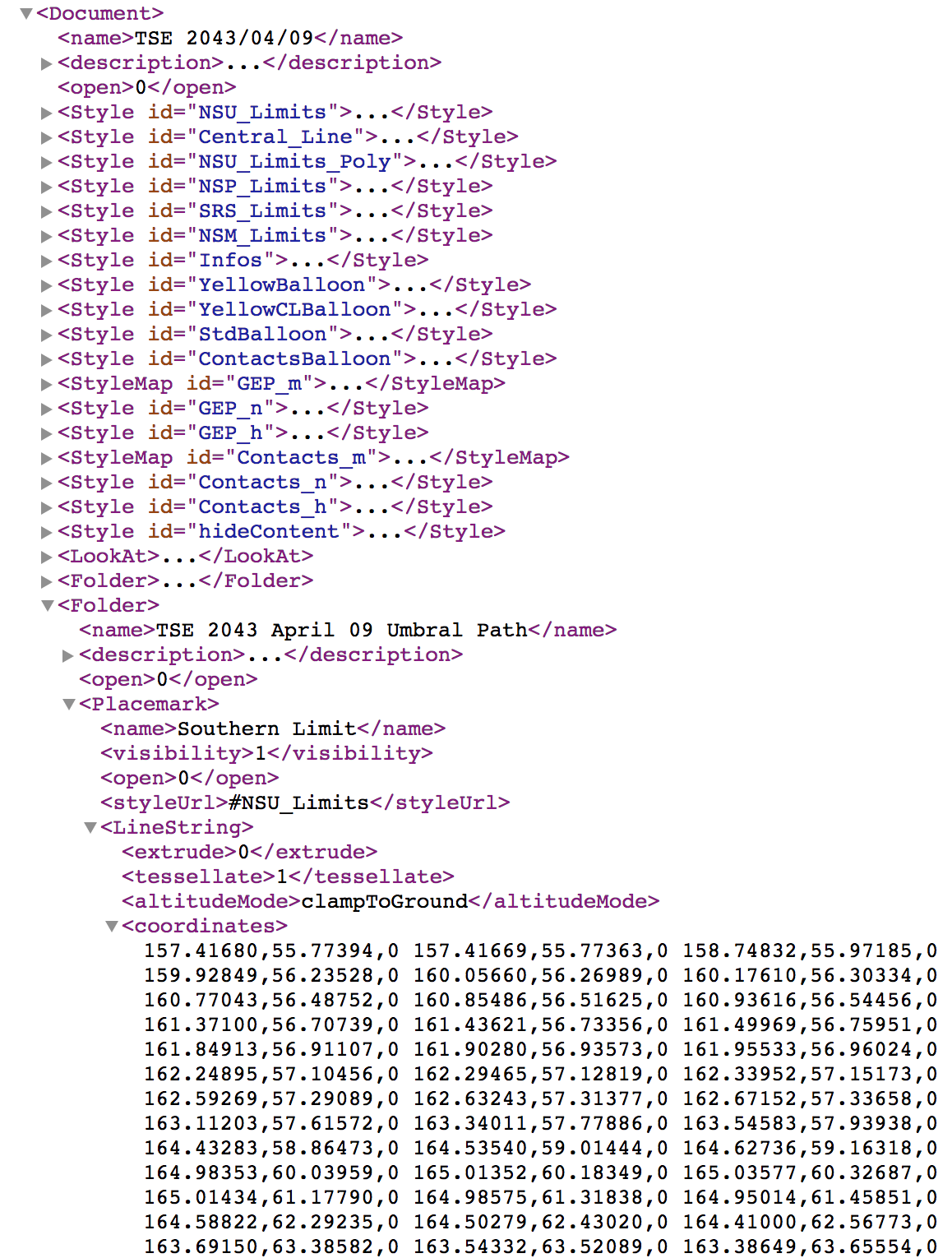
More bad news: if I take a look at the file_name.kml file, I’ll see a file structure that at first seems very difficult to understand.
Step 2: Extract eclipse data.
Good news: no one shouldn’t be intimidated by kml. After a few minutes I was quick to recognize that all data were contained under the “<Document><Folder>” path. In each folder is a different layer that could be mapped. In the case of my visualization I was interested in the Umbral Path which was described in <name> tag. This is the path of totality. Within the <Folder> structure there are three different <Placemark> tags: Norther Limit, Center Line, and Southern Limit. Within the <Placemark> tag there are <coordinates> in which I could extract.
This is just a long-winded way of saying there is a consistent path we can follow to extract coordinates. All we need to do is extract this information. I prefer R, so here is a little function I wrote to pull the data. I’m also going to show a long function but its commented out so I can see what is done. This is also half of all the code needed to create the file.
# Build a function to extract coordinates.
# input folder location into function.
extract_data <- function(loc = "/Users/luke.stanke/Downloads//TSE_2038_12_26.kmz") {

# Find kml file.
  loc <-
    loc %>%
    list.files() %>%
    .[!stringr::str_detect(., "files")] %>%
    paste(loc, ., sep = "/")

# Read .kml.
  shape <- xml2::read_html(loc)


# Get data for the Umbral Path folder.
  valid <-
    shape %>%
    rvest::html_nodes("folder") %>%
    stringr::str_detect(., "Umbral Path")

# Extract coordinates.
  shape_file <-
    shape %>%
    rvest::html_nodes("folder") %>%
    .[valid] %>%
    rvest::html_nodes("placemark linestring coordinates") %>%
    .[1] %>%
    rvest::html_text("") %>%
    stringr::str_replace_all("\r", "") %>%
    stringr::str_trim() %>%
    stringr::str_split(" ") %>%
    unlist() %>%
    data_frame(
      coords = .
    )

# Pull data for the Southern Limit.
  name <-
    shape %>%
    rvest::html_nodes("folder") %>%
    .[valid] %>%
    rvest::html_nodes("placemark name") %>%
    .[1] %>%
    rvest::html_text()

# Build the data frame.
  shape_file <-
    strsplit(shape_file$coords, ",") %>%
    unlist() %>%
    matrix(ncol = 3, byrow = TRUE) %>%
    as_data_frame %>%
    mutate(
      V1 = as.numeric(V1),
      V2 = as.numeric(V2),
      V3 = as.numeric(V3),
      name = name
    ) %>%
    rename(
      latitude = V1,
      longitude = V2,
      altitude = V3
    ) %>%
    tibble::rownames_to_column("index")

# Repeat for Central Line.
  if(shape %>%
    rvest::html_nodes("folder") %>%
    .[valid] %>%
    rvest::html_nodes("placemark linestring coordinates") %>%
    length() %>%
    `>=`(2)) {

    shape_file2 <-
      shape %>%
      rvest::html_nodes("folder") %>%
      .[valid] %>%
      rvest::html_nodes("placemark linestring coordinates") %>%
      .[2] %>%
      rvest::html_text("") %>%
      stringr::str_replace_all("\r", "") %>%
      stringr::str_trim() %>%
      stringr::str_split(" ") %>%
      unlist() %>%
      data_frame(
        coords = .
      )

    name <-
      shape %>%
      rvest::html_nodes("folder") %>%
      .[valid] %>%
      rvest::html_nodes("placemark name") %>%
      .[2] %>%
      rvest::html_text()

    shape_file2 <-
      strsplit(shape_file2$coords, ",") %>%
      unlist() %>%
      matrix(ncol = 3, byrow = TRUE) %>%
      as_data_frame %>%
      mutate(
        V1 = as.numeric(V1),
        V2 = as.numeric(V2),
        V3 = as.numeric(V3),
        name = name
      ) %>%
      rename(
        latitude = V1,
        longitude = V2,
        altitude = V3
      ) %>%
      tibble::rownames_to_column("index")

    shape_file %<>%
      bind_rows(shape_file2)


  }

# Repeat for Northern Limit.
  if(shape %>%
     rvest::html_nodes("folder") %>%
     .[valid] %>%
     rvest::html_nodes("placemark linestring coordinates") %>%
     length() %>%
     `>=`(3)) {

    shape_file2 <-
      shape %>%
      rvest::html_nodes("folder") %>%
      .[valid] %>%
      rvest::html_nodes("placemark linestring coordinates") %>%
      .[3] %>%
      rvest::html_text("") %>%
      stringr::str_replace_all("\r", "") %>%
      stringr::str_trim() %>%
      stringr::str_split(" ") %>%
      unlist() %>%
      data_frame(
        coords = .
      )

    name <-
      shape %>%
      rvest::html_nodes("folder") %>%
      .[valid] %>%
      rvest::html_nodes("placemark name") %>%
      .[3] %>%
      rvest::html_text()

    shape_file2 <-
      strsplit(shape_file2$coords, ",") %>%
      unlist() %>%
      matrix(ncol = 3, byrow = TRUE) %>%
      as_data_frame %>%
      mutate(
        V1 = as.numeric(V1),
        V2 = as.numeric(V2),
        V3 = as.numeric(V3),
        name = name
      ) %>%
      rename(
        latitude = V1,
        longitude = V2,
        altitude = V3
      ) %>%
      tibble::rownames_to_column("index")

    shape_file %<>%
      bind_rows(shape_file2)


  }

# Combine everything together.


  shape_file %>%
    rename(longitude = latitude, latitude = longitude) %>%
    mutate(index = as.numeric(index)) %>%
    filter(name != "Central Line") %>% # Chose to drop Central line later.
    mutate(
      index = ifelse(name == "Northern Limit", -index, index),
      index = ifelse(name == "Northern Limit", index, index),
      Date = loc %>%
        stringr::str_split("TSE_") %>%
        .[[1]] %>%
        .[2] %>%
        stringr::str_replace_all(".kml", "") %>%
        stringr::str_replace_all("_", "-") %>%
        lubridate::ymd()
    ) %>%
    arrange(index)
}
With this function we can quickly build the a single data frame with all of the eclipse data.
# Search for all TSE files in the Downloads folder.
key_dirs <-
  list.dirs("/Users/luke.stanke/Downloads/") %>%
  .[stringr::str_detect(., "TSE_")] %>%
  .[!stringr::str_detect(., "files")]

# Run a for loop to create data.
for(i in 1:length(key_dirs)) {
  if(i == 1) {
    eclipse <- extract_data(key_dirs[i])
  } else {
    eclipse %<>%
      bind_rows(
        extract_data(key_dirs[i])
      )
  }
}
This produces a data frame with latitude, longitude, altitude (just 1), index (for the path of the polygons) and date of eclipse.
Step 3: Build Projections.
If we quickly visualize this here’s what we’ll have.
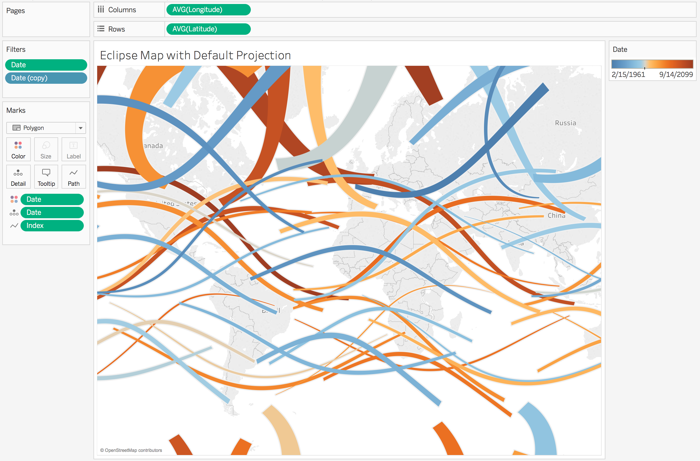
This is nice, but I really want this projected to look like a globe or Orthographic projection. To do this I need to create the math for the projection. We’re going to create 3 calculations in Tableau: [x], [y], and a filter called [valid]. We’ll first create two parameters: a base latitude and a base longitude. This will be our reference point that allows us to move around the globe.
The [Base Longitude] parameter is set to a range of -180 to 180 with steps of 15 degrees. This will eventually rotate the globe clockwise or counter-clockwise.

The [Base Latitude] parameter is set to a range of -90 to 90 with steps of 15 degrees. This will tilt the globe up or down towards the poles.

With these, let’s build our [x], [y], and [valid] calculations for the globe projection (we’re going to edit these later). X and Y will identify the new coordinates, while valid will work as a filter to only show values that are on facing outward from the projection.
// In Tableau: Create X coordinates.
COS(RADIANS([Latitude])) * SIN(RADIANS([Longitude]) - RADIANS([Base Longitude]))
// In Tableau: Create Y coordinates.
(
  COS(RADIANS([Base Latitude])) *
  SIN(RADIANS([Latitude]))
) - (
  SIN(RADIANS([Base Latitude])) *
  COS(RADIANS([Latitude])) *
  COS(RADIANS([Longitude]) - RADIANS([Base Longitude]))
)
// In Tableau: Valid filter.
(
  SIN(RADIANS([Base Latitude])) *
  SIN(RADIANS([Latitude]))
) + (
  SIN(RADIANS([Base Latitude])) *
  SIN(RADIANS([Latitude])) *
  COS(RADIANS([Longitude]) - RADIANS([Base Longitude]))
)
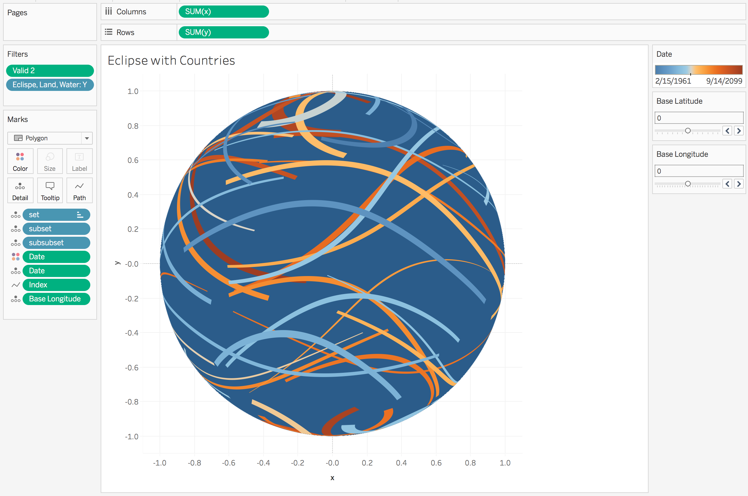
Here is what I should see if I add [x] and [y] to the columns and rows, add date to color and index to path, and add [valid] to filter and set the range from 0 to 1.
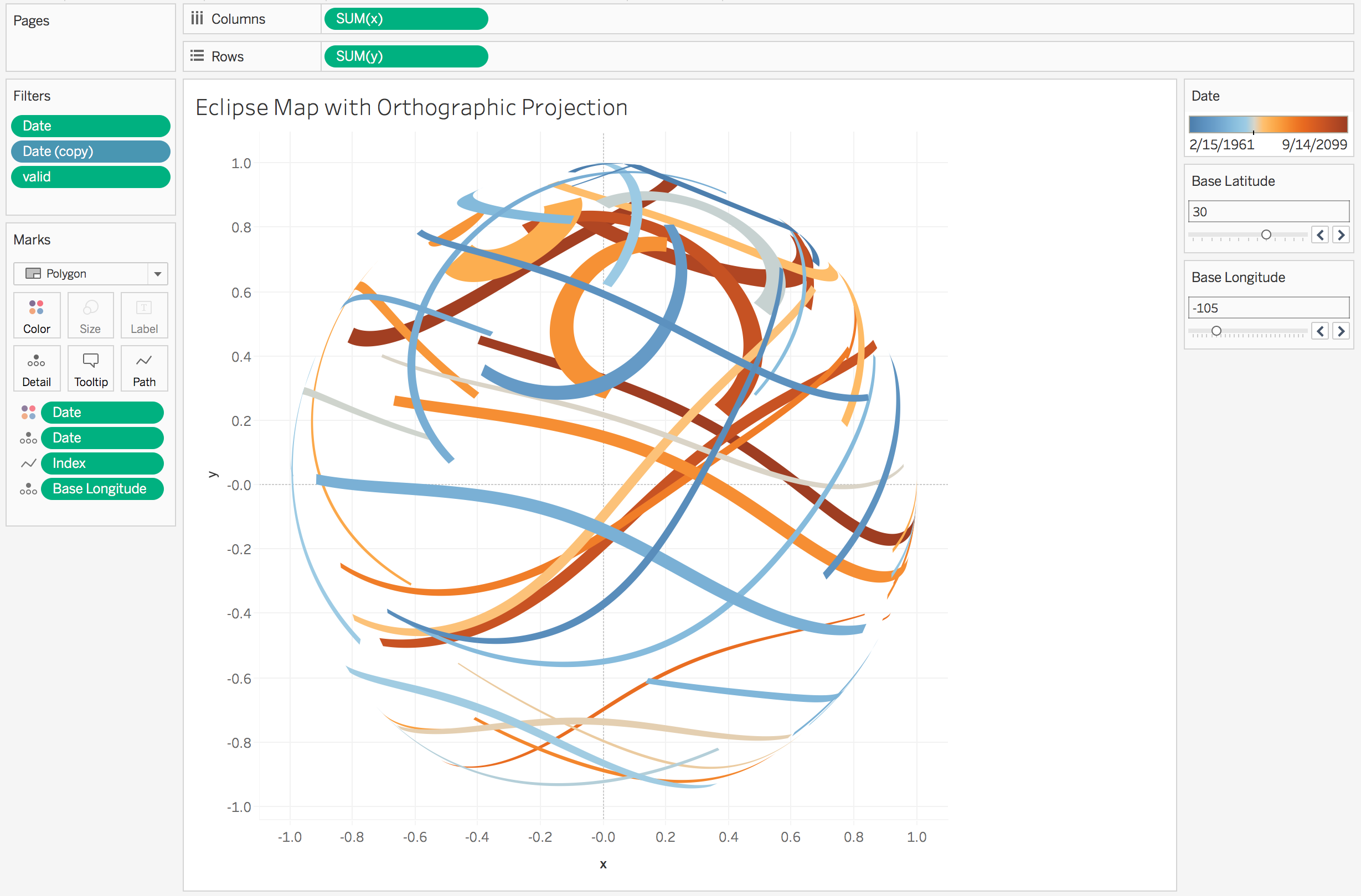
Boom! its the eclipses projected to a sphere. Once again, bad news: we don’t have the earth behind the globe. But we can find this data and append it to the existing dataset.
Step 4: Download and extract shapefiles of countries.
In my opinion the go-to file is “ne_10m_admin_0_countries_lakes.shp”. This is country boundaries without lakes at 10 meters. Basically it’s far more detailed than we probably need but its nice. Just give it a search on the web and download the file.
Data are easily read into R with the st_read() function and polygon data can be extracted with the st_geometry() function.
When taking a look at the data this point I notice data are MULTIPOLYGON. The best way to describe this is that each country is made up of multiple polygons (potentially) therefore each country is has a set of polygons nested within each country. In some cases these polygons are nested multiple levels deep. A little investigation in the data told me there were three levels. Being the creative type I named each of these levels “set”, “subset”, and “subsubset”.
# Read in Land data.
library(sf)
land <- st_read("/Users/luke.stanke/Downloads/ne_10m_admin_0_countries_lakes/ne_10m_admin_0_countries_lakes.shp")

# Obtain underlying geometry/shapes.
land <- st_geometry(land)

# Get underlying data in shapefiles.
# ADMIN, ABBREV are Labels.
# scalerank, LABELRANK, TINY are admin levels I considered as filters.
land_data2 <-
  land %>%
  as.data.frame() %>%
  select(scalerank, LABELRANK, ADMIN, ABBREV, TINY) %>%
  as_data_frame()


# Create empty data frame to load data into.
land_data <-
  data_frame(
    longitude = double(),
    latitude = double(),
    set = character(),      # Data are nested.
    subset = character(),   # These are nesting
    subsubset = character() # identifiers.
  )
From there it’s a matter of looping through the layers to extract the data
# sort through highest level (countries).
for(i in 1:length(land)) {
  level_1 <-
    land %>%
    .[[i]] %>%
    stringr::str_split("MULTIPOLYGON \\(")

  # Sort through second level. (subset)
  for(j in 1:length(level_1)) {
    level_2 <-
      level_1 %>%
      .[[j]] %>%
      stringr::str_split("list\\(") %>%
      .[[1]] %>%
      .[. != ""] %>%
      stringr::str_split("c\\(") %>%
      .[[1]] %>%
      .[. != ""]

# Sort through third level get data and add to dataframe. (subsubset)
    for(k in 1:length(level_2)) {
      level_2 %>%
        .[k] %>%
        stringr::str_replace_all("\\)", "") %>%
        stringr::str_split(",") %>%
        .[[1]] %>%
        stringr::str_trim() %>%
        as.numeric() %>%
        .[!is.na(.)] %>%
        matrix(ncol = 2) %>%
        as_data_frame() %>%
        rename(
          longitude = V1,
          latitude = V2
        ) %>%
        mutate(
          set = i,
          subset = j,
          subsubset = k
        ) %>%
        bind_rows(land_data) ->
        land_data
    }
  }
}

# Sort data by set, subset, subsubset.
land_data %<>%
  arrange(set, subset, subsubset)

# Join underlying data.
land_data %<>%
  mutate(set = as.character(set)) %>%
  left_join(
    as_data_frame(land_data2) %>%
    tibble::rownames_to_column("set")
  )

land_data %<>%
  mutate(
    name = "Land",
    altitude = 1
  ) %>%
  group_by(set, subset) %>%
  mutate(
    index = row_number()
  )
This produces a dataset with columns of latitude, longitude, set, subset, and subsubset. Now all we need to do is join this data together.
eclipse %<>%
  mutate(altitude = 1.01) %>%
  bind_rows(land_data)

# Write file.
eclipse %>%
  readr::write_csv("eclipse.csv")
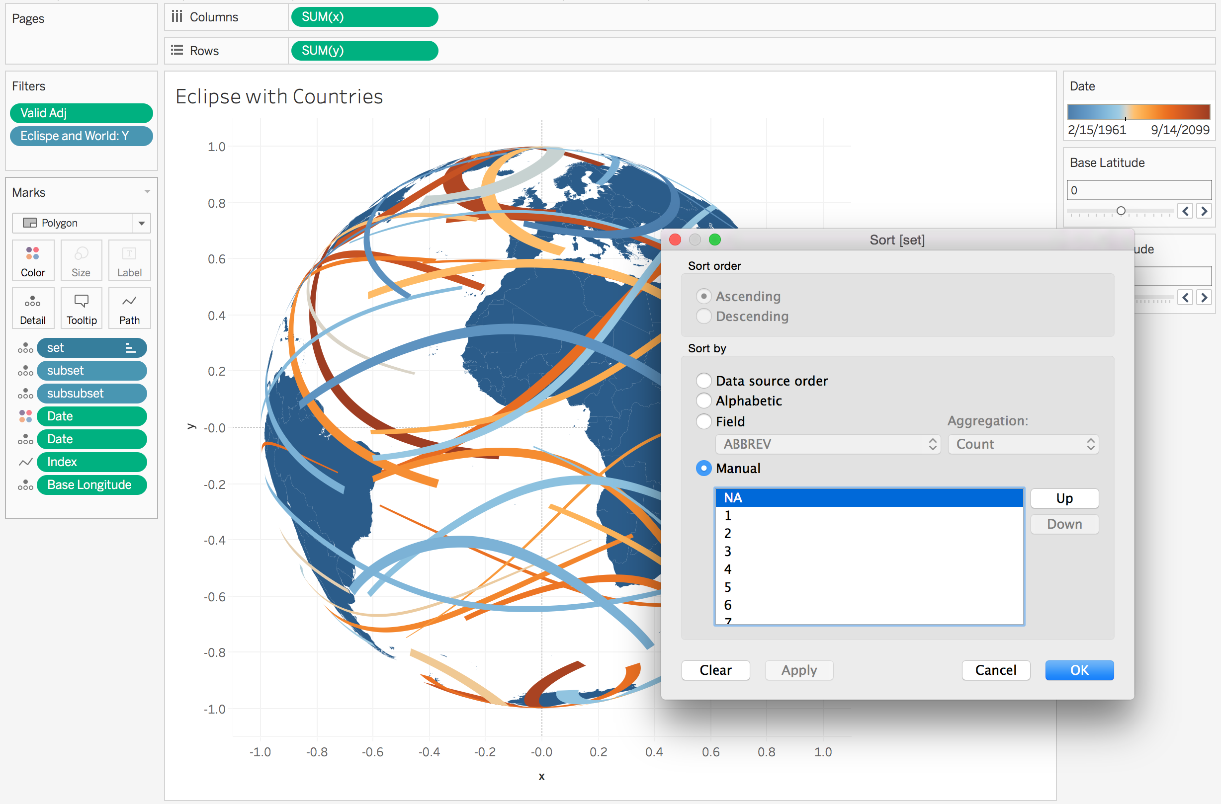
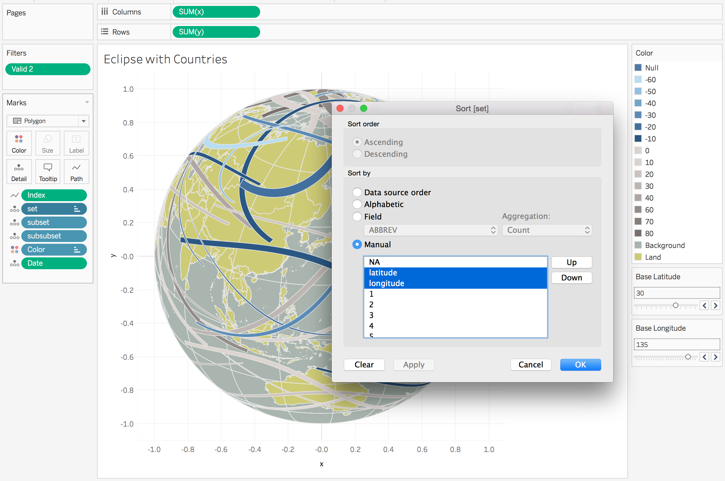
If I go back to Tableau and refresh my data, add [set], [subset], and [subsubset] to detail, I now have countries.
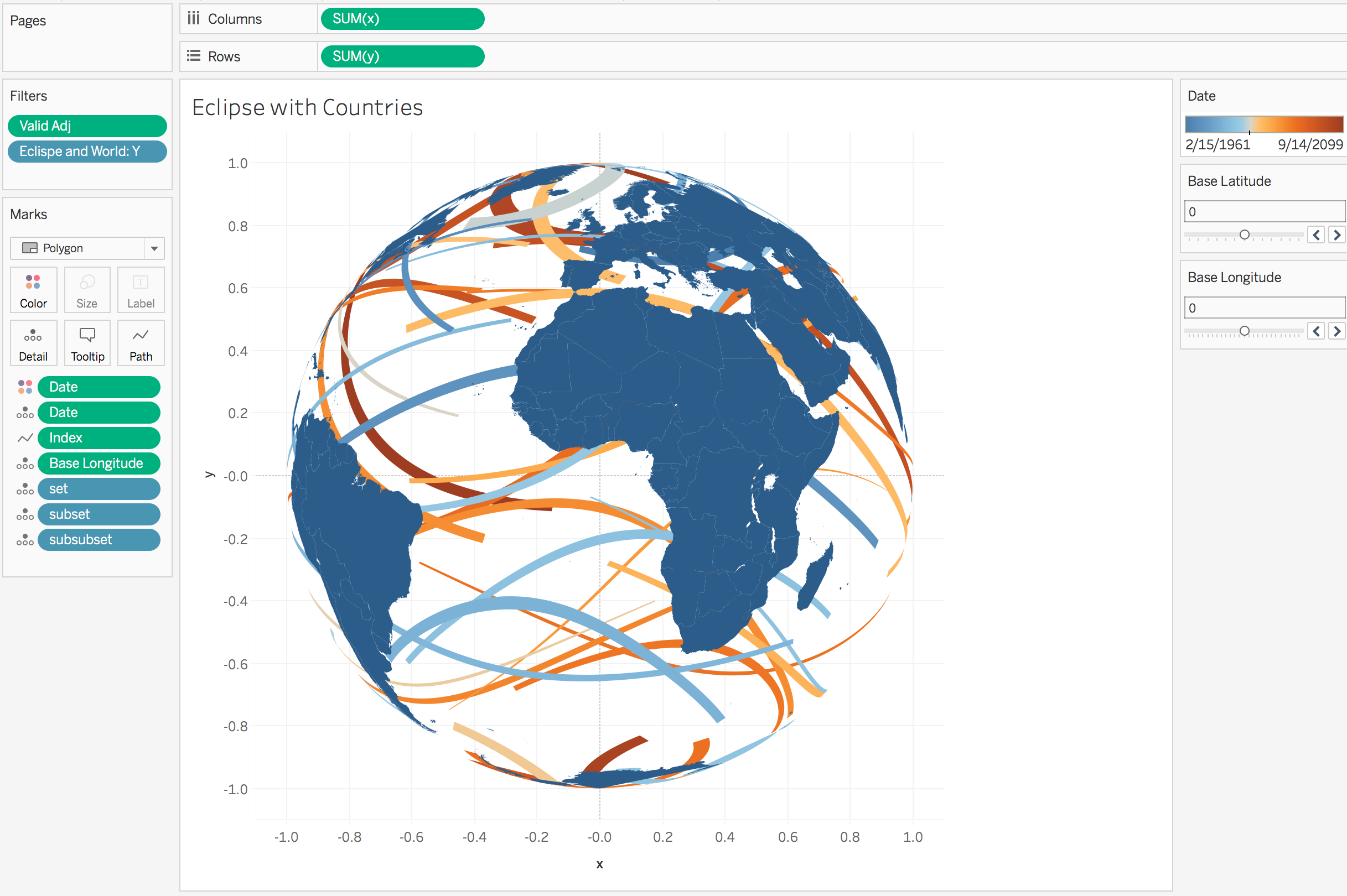
To place countries in the right order we need to a manual sort the [set] dimension placing “NA” at the highest level of the sort screen.
Step 5: Edit functions to encorporate great circle (globe background).
Things are starting to look good. Even with a little formatting I could be done there. But what I want is a background of ocean – or a great circle – representing the boundaries of earth. I’m going to use the following R code to build my great circle:
# Build great circle.
outline <-
  data_frame(
    index = seq(0, 360, 1/3),
    altitude = 1,
    set = "Outline" # Create a data point every 1/3 of a degree.
  ) %>%
  mutate(
    latitude = altitude * cos(2*pi*(index/360)),
    longitude = altitude * sin(2*pi*(index/360)),
    index = index*3
  )
This produces a dataset with five columns: [index], [altitude], [set], [latitude], and [longitude]. Once we have this dataset all we need to do is bind the data to our current eclipse data in R.
# Write file.
eclipse %>%
  bind_rows(outline) %>%
  readr::write_csv("eclipse.csv")
Step 6: Incorporate great circle in Tableau.
So here’s the thing. For the outline data in R, I already set the latitude and longitude to the appropriate projections in Tableau, meaning if I apply the projections again – which would happen if I left the calculations in Tableau the same – I wouldn’t the the values I want because they would have been applied twice. This means I don’t ever want my current functions for the background to change. Which means I don’t want Tableau to apply the functions that I’ve already created for [x], [y], and [valid] when [set] is equal to “Outline”. Your probably wondering why I did it this way. Well one option would be to take this amount of points (360*3) and multiply it by (180*3) so that I don’t have to touch my current functions but that would bring in much more data than is necessary. Because I am bringing in only the outline, and I don’t want the outline to rotate as I change the projection, I need to edit/re-build my functions to support this particular situation.
Here is what the [x], [y], and [valid] functions should now look like:
// In Tableau: Edit X coordinates.
IF [set] = "Outline"
THEN [Longitude]
ELSE
    COS(RADIANS([Latitude])) *
    SIN(RADIANS([Longitude]) -
    RADIANS([Base Longitude]))
END
// In Tableau: Edit Y coordinates.
//COS(RADIANS([Latitude])) * SIN(RADIANS([Longitude]))
IF [set] = "Outline"
THEN [Latitude]
ELSE
  (
    COS(RADIANS([Base Latitude])) *
    SIN(RADIANS([Latitude]))
  ) - (
    SIN(RADIANS([Base Latitude])) *
    COS(RADIANS([Latitude])) *
    COS(RADIANS([Longitude]) - RADIANS([Base Longitude])))
END
// In Tableau: Edit valid coordinates.
IF [set] = "Outline"
THEN [Latitude]
ELSE
  (
    SIN(RADIANS([Base Latitude])) *
    SIN(RADIANS([Latitude]))
  ) + (
    COS(RADIANS([Base Latitude])) *
    COS(RADIANS([Latitude])) *
    COS(RADIANS([Longitude]) - RADIANS([Base Longitude]))
  )
END
From the re-worked functions above you should see that we are basically skipping the application of the the projections to the great circle – which is exactly what we wanted to do. When we then take a look at our visualization, we have the following:
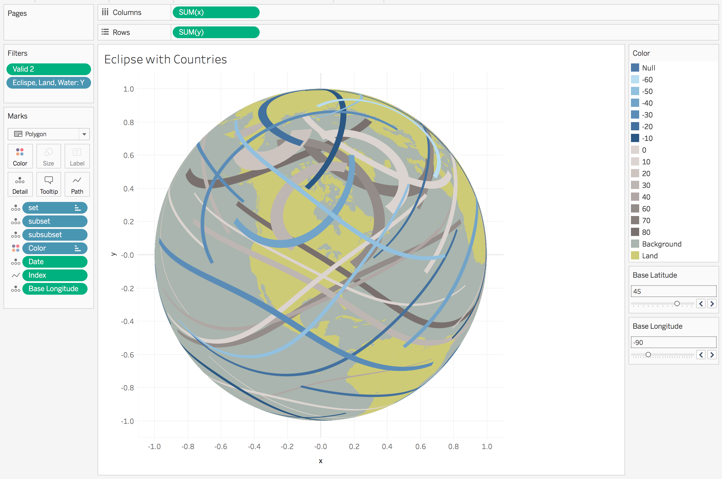
There is no issue with the visualization, the countries are just the same color as the background. Lets create a crude color palette to color everything in how we would like:
// In Tableau: Create [color] dimension.
IF [set] = "Background"
THEN "Background"
ELSEIF [ADMIN] != "NA"
THEN "Land"
ELSE STR(-ROUND([Years]/10)*10) // Group eclipses by 10 year occurrences.
END
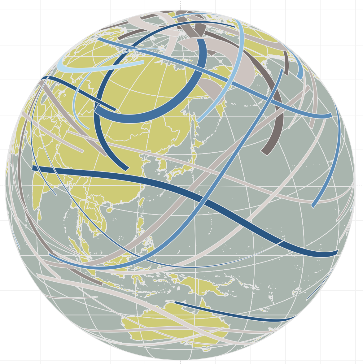
Dropping this new color calculation onto the color mark should produce something like this:
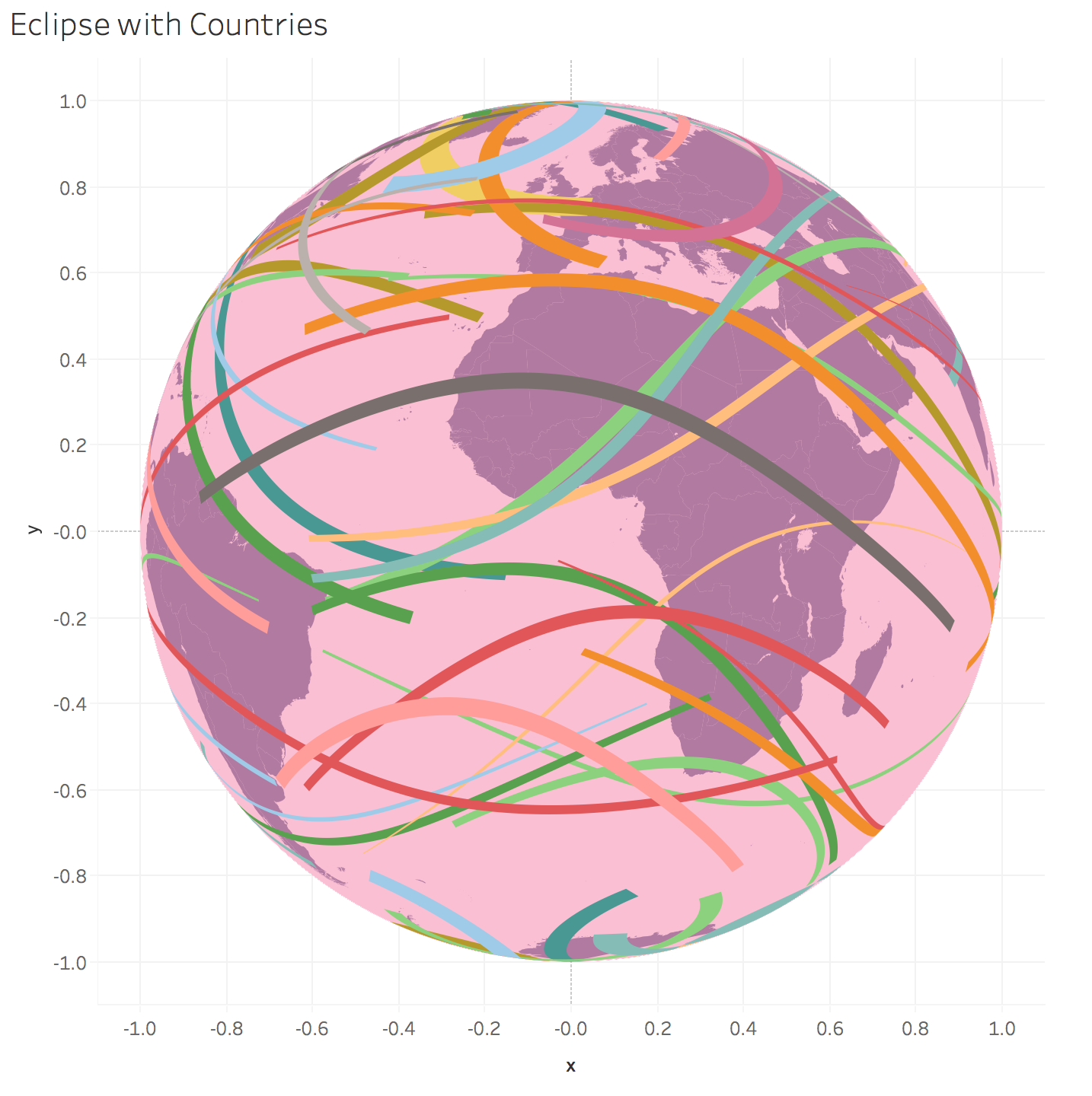
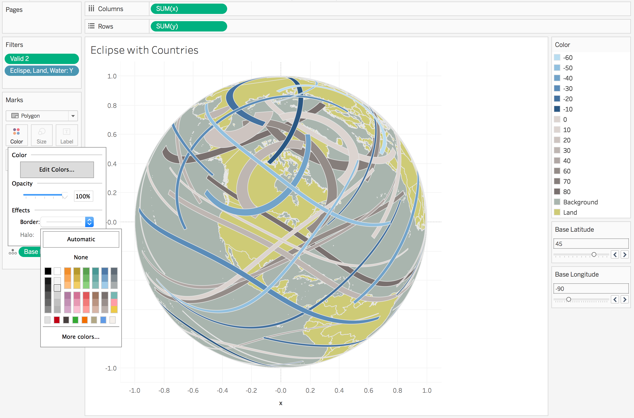
From there a little customization of the color can produce the following:
If I wanted to show the outline of the countries and the eclipse polygons all I need to do is add a border to the color.
Step 7: Create lines of latitude and longitude to add to the map.
Okay, this is the hardest thing to do of the map. Up until now it was basically get the data, create projections, edit data, edit projections, , re-edit data, re-edit projections. Now what I want to do is add grid lines for latitude and longitude. Here’s the thing: our current visualization is made up of polygons. I cant mix-and-match my to have both lines and polygons. This means I need to make the lines into polygons. This means draw each latitude and longitude line and then trace the same path backwards until I am back where I started the line. Then I basically have a polygon with no surface between the edges.
Here’s the R code to create the latitude and longitude “polygons”:
# Build latitude/longitude polygons.
# Build latitude.
latitude <-
  c(seq(0, 90, 20), -seq(0, 90, 20)) %>%
  sort() %>%
  unique() %>%
  rep(each = 360)

longitude_ <-
  -179:180 %>%
  rep(length(unique(latitude)))

latitude <-
  data_frame(
    latitude = latitude,
    longitude = longitude_,
    altitude = 1,
    index = longitude_,
    set = "latitude",
    subset = latitude
  )

latitude %<>%
  bind_rows(
    latitude %>%
      mutate(index = 361 - index)
  )

# Build longitude.
longitude <-
  seq(-180, 179, 20) %>%
  rep(each = length(seq(-90, 90, 1)))

latitude_ <-
  seq(-90,90, 1) %>%
  rep(length(seq(-180, 179, 20)))

longitude <-
  data_frame(
    longitude = longitude,
    latitude = latitude_,
    altitude = 1,
    index = latitude_,
    set = "longitude",
    subset = longitude
  )

longitude %<>%
  bind_rows(
    longitude %>%
      mutate(
        index = 361 - index
      )
  )

# Output FINAL .csv
eclipse %>%
  bind_rows(latitude) %>%
  bind_rows(longitude) %>%
  bind_rows(outline) %>%
  readr::write_csv("eclipse.csv")
This is the last time I’ll use R and export data from it. Now we can just refresh our dataset in Tableau you’ll see the following:
Step 8: Fix the latitude lines.
Everything looks nearly correct except for the lines connecting the ends of the latitude lines. If you rotate the map you’ll see sometimes they show up and other times they do not. The short description reason is they show up when the start of each latitude line is in the current visible space. When we apply the valid filter, instead of looping back on itself (remember the latitude polygon is designed to go all the way around then trace back on the loop to the star. The fix is simple: we need the start of each latitude line by adjusting the [longitude] function to start on the opposite side of the current visible earth. This will allow for correct clipping.
I’ll create a new function called [Long Adj] to represent the adjusted longitude
// In Tableau: Create [long adj] measure.
IF CONTAINS([set], "latitude")
THEN [Longitude] + [Base Longitude]
ELSE [Longitude]
END
With this new longitude calculation, we then need to edit the [x], [y], and [valid] functions one last time.
// In Tableau: Edit X coordinates.
IF [set] = "Outline"
THEN [Longitude]
ELSE
    COS(RADIANS([Latitude])) *
    SIN(RADIANS([Long Adj]) -
    RADIANS([Base Longitude]))
END
// In Tableau: Edit Y coordinates.
//COS(RADIANS([Latitude])) * SIN(RADIANS([Long Adj]))
IF [set] = "Outline"
THEN [Latitude]
ELSE
  (
    COS(RADIANS([Base Latitude])) *
    SIN(RADIANS([Latitude]))
  ) - (
    SIN(RADIANS([Base Latitude])) *
    COS(RADIANS([Latitude])) *
    COS(RADIANS([Long Adj]) - RADIANS([Base Longitude])))
END
// In Tableau: Edit valid coordinates.
IF [set] = "Outline"
THEN [Latitude]
ELSE
  (
    SIN(RADIANS([Base Latitude])) *
    SIN(RADIANS([Latitude]))
  ) + (
    COS(RADIANS([Base Latitude])) *
    COS(RADIANS([Latitude])) *
    COS(RADIANS([Long Adj]) - RADIANS([Base Longitude]))
  )
END
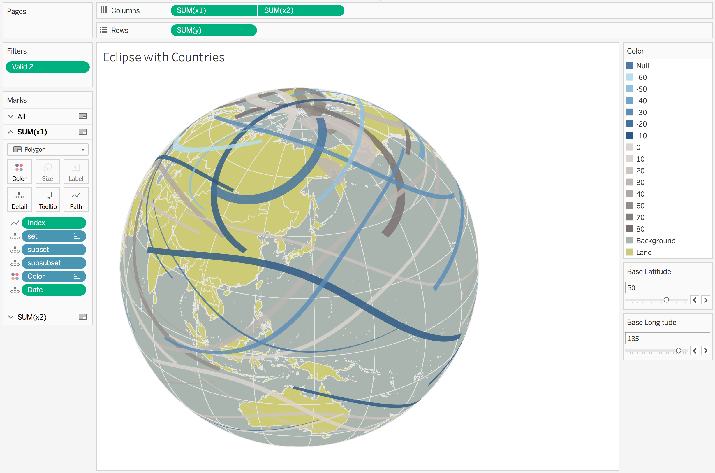
These updates produces the following visualization after you re-sort the [set] values of “latitude” and “longitude” just below “NA” :
Step 9: Add borders to countries and keep latitude/longitude lines.
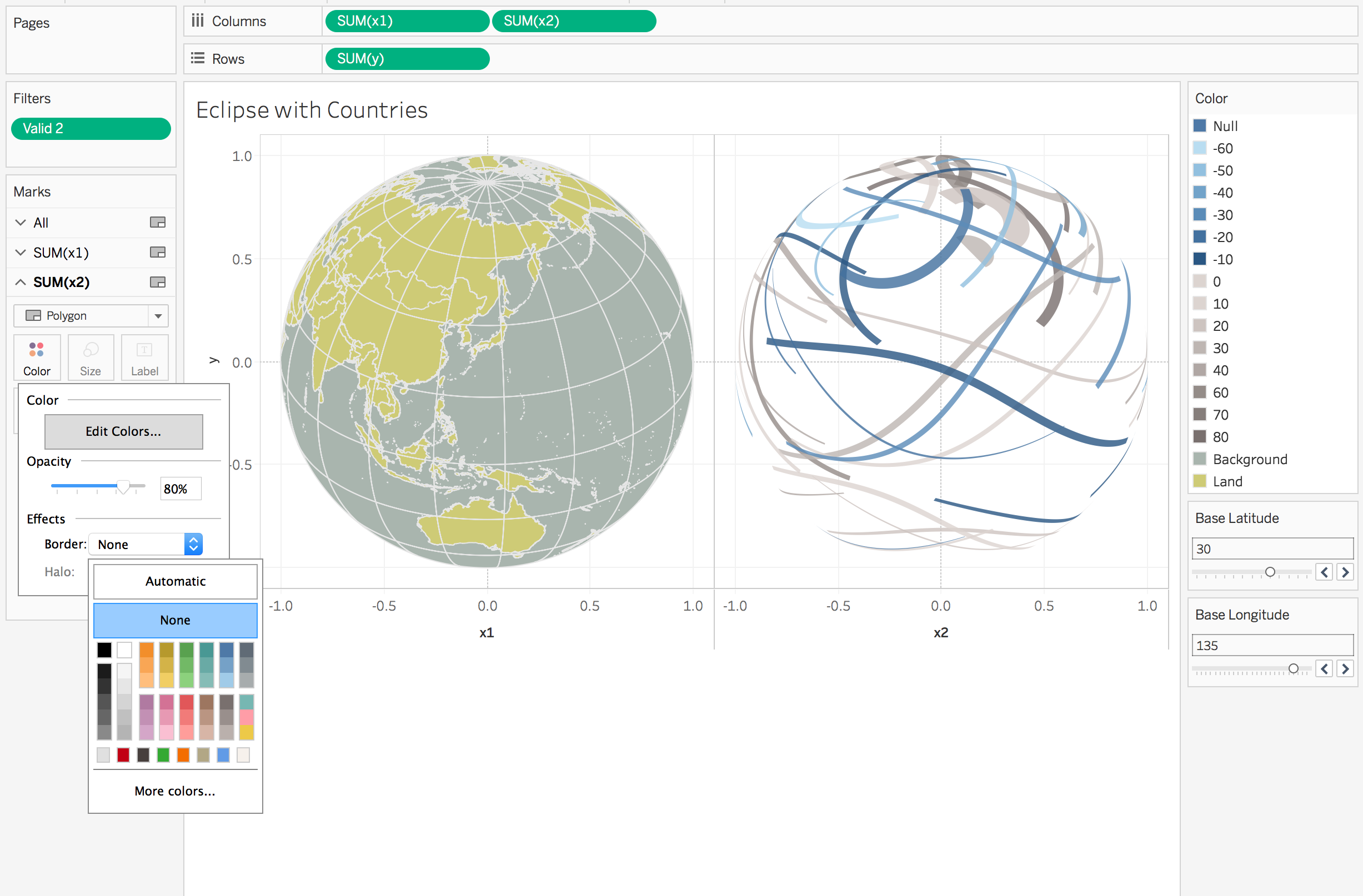
Now this looks really good. The only difference is I want my eclipse polygons not to have outlines and for every country to have borders and latitude/longitude grid lines to show up.
This requires me to create two x calculations and then create a dual axis chart.
My new x calculations – [x1] and [x2] are then:
// In Tableau: Create [x1] calculation for everything but eclipses.
IF ISNULL([Date])
THEN [x]
END
// In Tableau: Create [x2] calculation for only eclipses.
IF NOT ISNULL([Date])
THEN [x]
END
I can now replace [x1] with [x] on the columns shelf and add [x2] the columns shelf. I’ll also edit the borders on [x2] and opacity of color.
Step 10: Clean things up.
From here all I need to do is create the dual axis chart, synchronize the axes, do some formatting, and remove tooltips.
And that’s it. Is there a lot of custom coding? Yes, to get the data of the eclipses. There was also a little work to get the multipolygons of each country. But now I have countries for future maps so there is little work involved to do this in the future. Was it hard? No. There are only a few calculations I have created in Tableau: [x] (and [x1] and [x2]), [y], [valid], [long adj], and the optional [color]. There were also 2 parameters that allowed me to rotate the map [Base Latitude] and [Base Longitude]. Given the 7 custom components I’d call this one easy but time intensive (to write the blog).